Tuning Bandits at Fleet Scale

What JustAI does. JustAI runs message optimization for consumer apps: the welcome emails, reminders, push notifications, and promotions they send their users. For each message, the customer gives us a few candidate versions and a goal, almost always a conversion like a purchase or a signup, and we decide which version to send, to whom, continuously and per audience, learning from real responses instead of a one-off A/B test. At any time we are running this across hundreds of campaigns for dozens of companies.

How it works. Picking which version to send is a decision under uncertainty: you only learn how good a version is by sending it, and every send spent probing a weak version is one you did not spend on the best one. That trade-off, explore to learn versus exploit what you know, is a multi-armed bandit, and it is the engine underneath. Each version is an arm, each send a pull, a conversion the reward. The system keeps an estimate of each version’s rate, sends the strong ones more often, and deliberately keeps sampling the rest so a good version is not buried by an unlucky start. Its objective is to lose as few conversions as possible against a chooser that always sends the best version, what we will later call regret. We do not run one bandit; we run thousands at once, one per message, and for personalized messages, one per audience segment.

What we were seeing. The algorithm is the easy part. The hard part is how a well-founded bandit degrades on real data: rewards are sparse and delayed, the audience splits into thousands of thin segments, and the best version drifts over time. Three failures stood out. On one onboarding email, a single mediocre version had held about 82% of all sends for six months while better versions sat starved of traffic. On a heavily personalized campaign, the audience was split so finely that most segments barely had the data to rank their versions, so allocation was close to random. And across the board, we were spending a fixed fraction of every message exploring alternatives long after the winner was settled.

Over the past few months we found and addressed this family of cases, upgrading the engine as we went, then built a novel system that catches the next one on its own. The rest of this post walks through each case and what we changed. One theme runs through all of them. The algorithm itself is sound; what’s complex is the tuning around it. A single set of defaults runs across thousands of campaigns and dozens of customers, and conditions vary enormously, so a one-size-fits-all decision engine would leave performance on the table for some of them.

The model we tune: weighted Thompson sampling

Everything we changed edits one model. For each metric it tracks (opens, clicks, conversions, unsubscribes), a variant keeps a Beta distribution over its rate: a running estimate that is wide when the variant has little data and narrow when it has a lot. To serve a request, the system draws one sample from each variant’s distribution per metric, combines the samples into a single score with the campaign’s weights, and sends the highest.

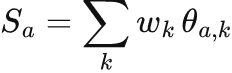
Here, θ_a,k is the rate sampled for variant a on metric k, and w_k is that metric's weight. Because each score uses a fresh random draw, a variant is sent in proportion to its probability of being best, a property called probability matching. It explores in proportion to its own uncertainty, and that exploration shrinks on its own as evidence accumulates. This is Thompson sampling, generalized to several weighted reward signals.

The piece that governs everything is the prior. Each metric’s prior is centered on the pool’s median rate μ with a strength of B pseudo-observations (default B = 1000), so a variant’s posterior mean (formed from c events of that metric over n sends, an observed rate c/n) is a shrinkage of that rate toward the field:

B is the dial. It sets how much evidence a variant must earn before the system trusts it over the crowd: a new variant is regularized toward the field instead of collapsing to zero, and a variant with n ≪ B stays effectively unranked. Much of what follows is choosing B, its center, and its variance for the data a variant actually has.

The objective, stated once: minimize cumulative regret over a horizon of T sends, the conversions lost against an oracle that always sends the best variant. Here ρ_a is each variant’s conversion rate and a_t the variant sent at step t:

Problem 1: one mediocre message held 82% of traffic for six months

One onboarding campaign was stuck. For six months our algorithm sent a single mediocre variant about 82% of the time while higher-converting variants starved below the exploration floor. Two changes to how the algorithm reads its own data, widening its uncertainty and correcting for good and bad days, broke the lock, surfaced the real winner, and lifted conversion +12.6% against a holdout. Here is why it happened and how the fix works. The point estimates were fine; the problem was the posterior variance, and it compounded from two sides.

The lock held for two reasons. New versions could not win enough traffic to prove themselves, and the current leader had gathered so much data that the system grew ever more certain about it and kept sending it. Here it is in detail. From below, the strong prior did the damage. With B = 1000 pseudo-observations, any challenger with n ≪ B stayed pinned near the pool median and effectively unranked, so probability matching almost never drew it, so it never earned the volume to escape the prior. From above, the incumbent had long since escaped: its posterior had contracted until its draws won the composite nearly every round, and exploitation bought the volume that contracted it further. A confident leader over a field of prior-starved challengers is a stable state that a small exploration floor cannot break. The fix had to widen variance and re-scale the base rate, not just add exploration.

So we widened each posterior without moving its mean: divide both Beta parameters α, β by a factor f. The mean is invariant and the variance inflates by a clean factor (with S = α + β) and coined it Effective Sample Size(ESS¹) Widening:

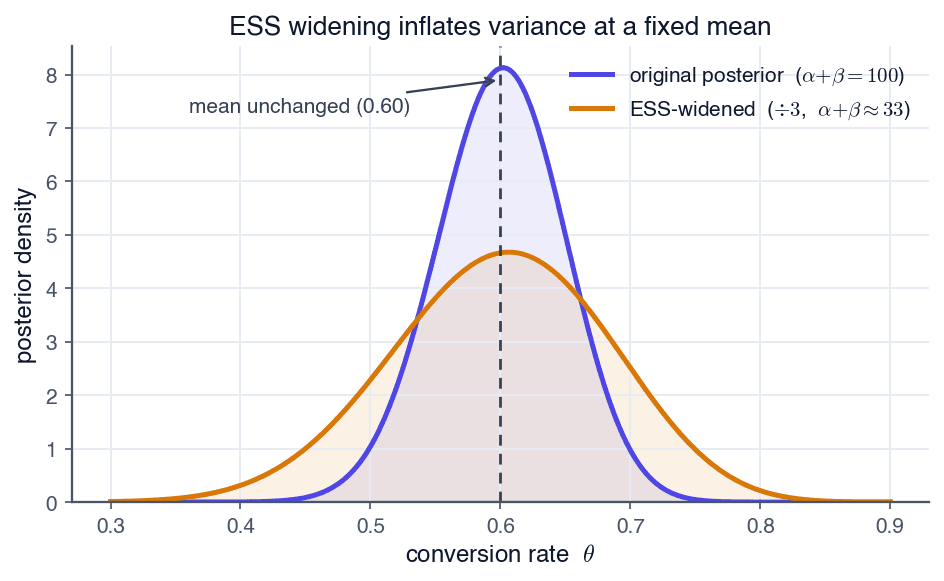
Figure 1: ESS widening

ESS widening on a single arm's Beta posterior: dividing both parameters by a factor holds the mean (dashed line) fixed and inflates the variance. A contracted leader loosens and starved challengers regain a fair sample, with no point estimate moved.

We paired it with pool normalization². Each variant’s daily counts c_a,d are rescaled by the ratio of the pool’s median daily rate r̄_med to its rate on that day r̄_d, pinning the pool’s daily rate to its median across days, applied only on days the pool clears 20 events:

Because variants are exposed on different sets of days, the correction is not the same for each variant: some days the whole platform converts more, so without it a variant could look best just for landing on those good days. Pinning each day to the pool’s median removes that timing edge, and because the day-sets differ, it can move the true winner back on top. On turn-on day the lock broke: the entrenched variant fell from 82% to about 5% and held, a previously-starved variant surfaced as the genuine best converter, and against a reserved holdout the change ran +12.6% (z = 4.3, p < 0.0001). The caveat we insisted on: widening is mean-preserving, so it only pays off when a lock came from over-confidence rather than a real gap. It can surface a starved winner, but it cannot manufacture one.

Problem 2: twenty-one thousand experiments, most too thin to call

One heavily personalized campaign was barely learning. Split into 21,394 segments across 30 variants, most segments saw too few sends to tell their variants apart, so allocation collapsed toward random: on the largest campaign the leading variant’s 7.3% share was almost exactly its uniform share. Letting the segments share what they learn, instead of each guessing alone, recovered about +18% conversion. Here is the failure and the fix. Split that finely, each segment’s maximum-likelihood rate is a high-variance estimate, and its allocation collapses toward uniform.

A fixed prior cannot escape the bias-variance bind: strong enough to tame the variance in segments and it erases the real differences between them; weak enough to keep the differences and it overfits the noise. So we stopped estimating each segment alone and let them borrow strength. In plain terms, a segment with little data mostly inherits how that version performs across the whole campaign, and it leans on its own numbers only as it collects enough of them. Concretely, we place a shared prior across segments and center each segment’s estimate on that variant’s own template-wide rate, weighted by how much evidence the segment has earned. This is empirical-Bayes partial pooling³, with one tunable parameter τ (here c indexes the segment, r̂_a,c is the segment’s own rate, and μ_a the variant’s template-wide rate):

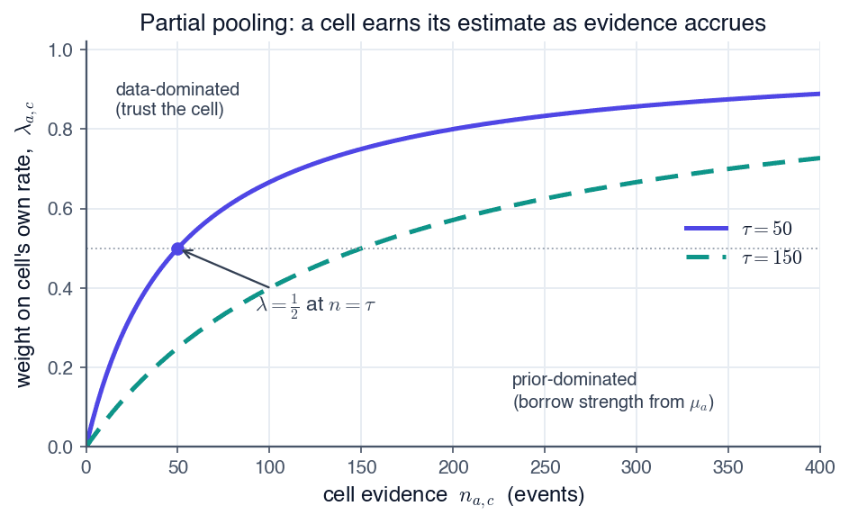
Figure 2: Shrinkage

Shrinkage: a segment earns its own estimate only as it accumulates evidence; until then it inherits the variant's template-wide rate.

The subtlety that made it work, and that a single global knob misses, is that the fix has two operating points. In near-empty segments the prior’s content is the only signal, so naively weakening the prior backfired and went negative on a thin template. The win came from making the prior informative: each variant inherits its own template-wide ranking into every segment, not a coin flip. Replayed on the 21,394-segment campaign, that recovered about +5,161 conversions/day, roughly +18%.

Discrete per-segment cells are themselves a stand-in. The principled version is a contextual bandit: model each variant’s reward as a function of the segment’s features, so strength is shared across similar segments automatically instead of pooled within hard-coded cells. Linear Thompson sampling (LinTS) is the standard form, and it is where this line of work points next.

Problem 3: a permanent exploration tax

Every campaign was paying a permanent exploration tax. A fixed ε-greedy floor randomized up to a quarter of all traffic forever, long after the winner was settled. Letting that floor shrink as evidence piles up recovered +3.5% to +10% conversion. Why it happened: a fixed floor is a linear regret tax. Because a fixed fraction of every send stays random, the wasted exploration grows with the total number of sends, a Θ(εT) term that never decays (Θ here is order-of-growth notation, not the rate θ), on top of Thompson sampling's own exploration, which fades on its own. So instead of a fixed floor, we let exploration start high and fade as evidence accumulates: it begins at a high rate ε₀ and decays with the observation count n over a scale of κ toward a small residual ε_min.

Integrating over the horizon shows the excess exploration above the residual is finite; it does not grow with T:

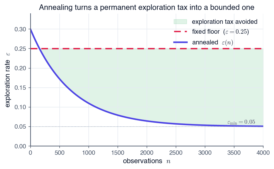
Figure 3: Epsilon annealing

A fixed ε floor is a permanent tax; annealing bounds the total exploration above the residual.

Annealing replaces the fixed floor’s Θ(εT) tax with a bounded O(κ) excess above the irreducible floor: the exploration you keep paying for becomes a deliberate residual rather than a function of the horizon. The payoff was stable across replications: +3.5% on one template, +10% on another.

The levers with sharp edges

The remaining fixes are lower on math and higher on stakes: each one helps in the setting it was meant for and hurts in the wrong one, so naming the sign-flip boundary was most of the work.

A weight is not its influence. A weight multiplies a rate, so a metric’s real contribution to the ranking is weight times typical rate, and rates differ about 60x across a standard config (opens ~33%, clicks ~0.6%). A weight of 10 on clicks therefore carries less pull than 1 on opens: the template was effectively ranking on opens while its stated objective was clicks. Sweeping the weight traces a U-shaped regret curve: zero throws away real signal, 100 is maximum variance, and a 5–20 plateau is the sweet spot. The principled version defines weights over pool-z-scored rates, so nominal weight equals influence by construction.

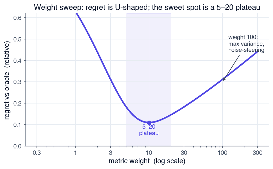
Figure 4: Weight sweep

The weight-sweep regret curve is U-shaped: zero throws away real signal, 100 is maximum variance, and a 5–20 plateau is the sweet spot.

Whether to demote is a correlation question, and we measure it. Before touching a heavily-weighted engagement metric we check whether it actually predicts the KPI: a per-variant Pearson correlation between the engagement rate and the conversion rate, read in bands. Aligned (r ≥ 0.3) means ranking on it is safe. Inverted (r ≤ −0.1) means ranking on it pulls against conversions. Both ends were real: one template’s engagement tracked its KPI at r ≈ 0.4, so the weight was safe; on another, a metric we had dismissed as too sparse turned out to be the one separating the variants, and demoting it starved the true best arm (its share fell 24% to 10%) before we caught it and reverted. Raw event count is not statistical power.

Some metrics cannot be a bandit objective at all. For a sub-1-event/day KPI, the per-arm sample size to detect a 20% minimum detectable effect⁴ (the 0.2 below) at 80% power is nearly rate-free. Here p is the KPI’s per-send rate and z_α/2, z_β the normal quantiles for 5% significance and 80% power:

That is about 450 days at 1 event/day and 7,000 days at 0.06. No allocation policy can optimize a target that resolves that slowly, so we rank on the plentiful signal and keep the sparse KPI as a report-only layer.

The levers interact, so we grade a change as one policy rather than one knob at a time. On a streaming-digest template, correcting which metric the bandit ranked on, by itself, graded −1.5%: fixing the objective bought nothing while a quarter of traffic was still randomized by a stale exploration floor. Co-tuned with the ε drop, the same weight fix graded +2.7 to +4.2%. Grading each knob independently on the live config misses exactly this coupling, so we replay a candidate as a whole configuration.

Making the bandit legible

The recurring blocker was concrete: we could not debug what we could not see. So we built a superadmin diagnostics stack on a faithful client-side mirror of the production scorer, with the same median-biased posteriors, composite, ε-greedy, and edge cases (an invalid non-positive-β posterior is marked rather than clamped into a fake spike).

A posterior chart renders each variant’s Beta per metric on any scoring day, with a slider over the template’s own history, so you can see which variant’s confidence is dominating.

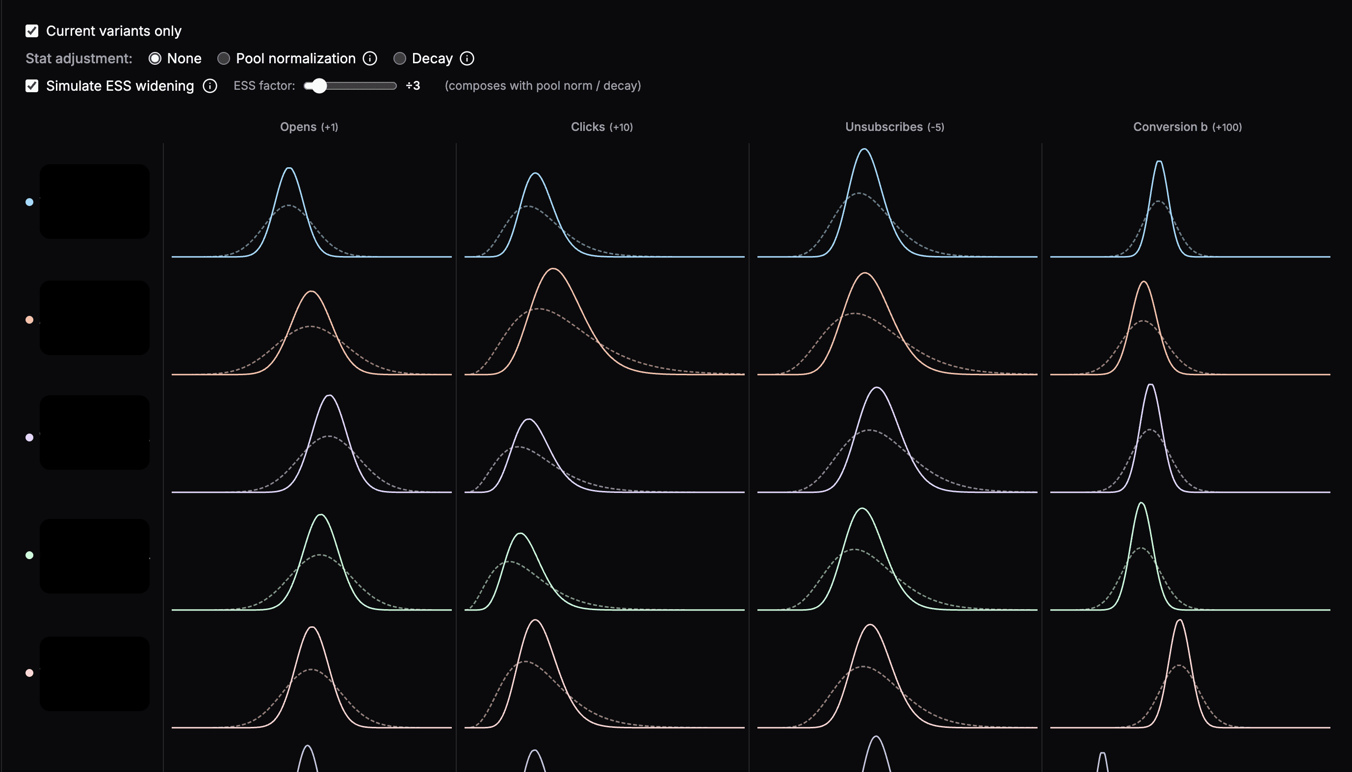
Figure 5: Posterior chart

The posterior chart: each variant's Beta posterior per scored metric (rows = variants, columns = metrics; variant names redacted). Solid = the live posterior, dashed = the same posterior under ESS widening.

A simulated send distribution estimates each variant’s probability of being optimal exactly as the live scorer does, by Monte Carlo: draw every variant’s posteriors M times, take the composite argmax on each draw, and count wins.

A what-if weights editor re-runs that same counterfactual under typed weights, on the template’s own history, before anything ships.

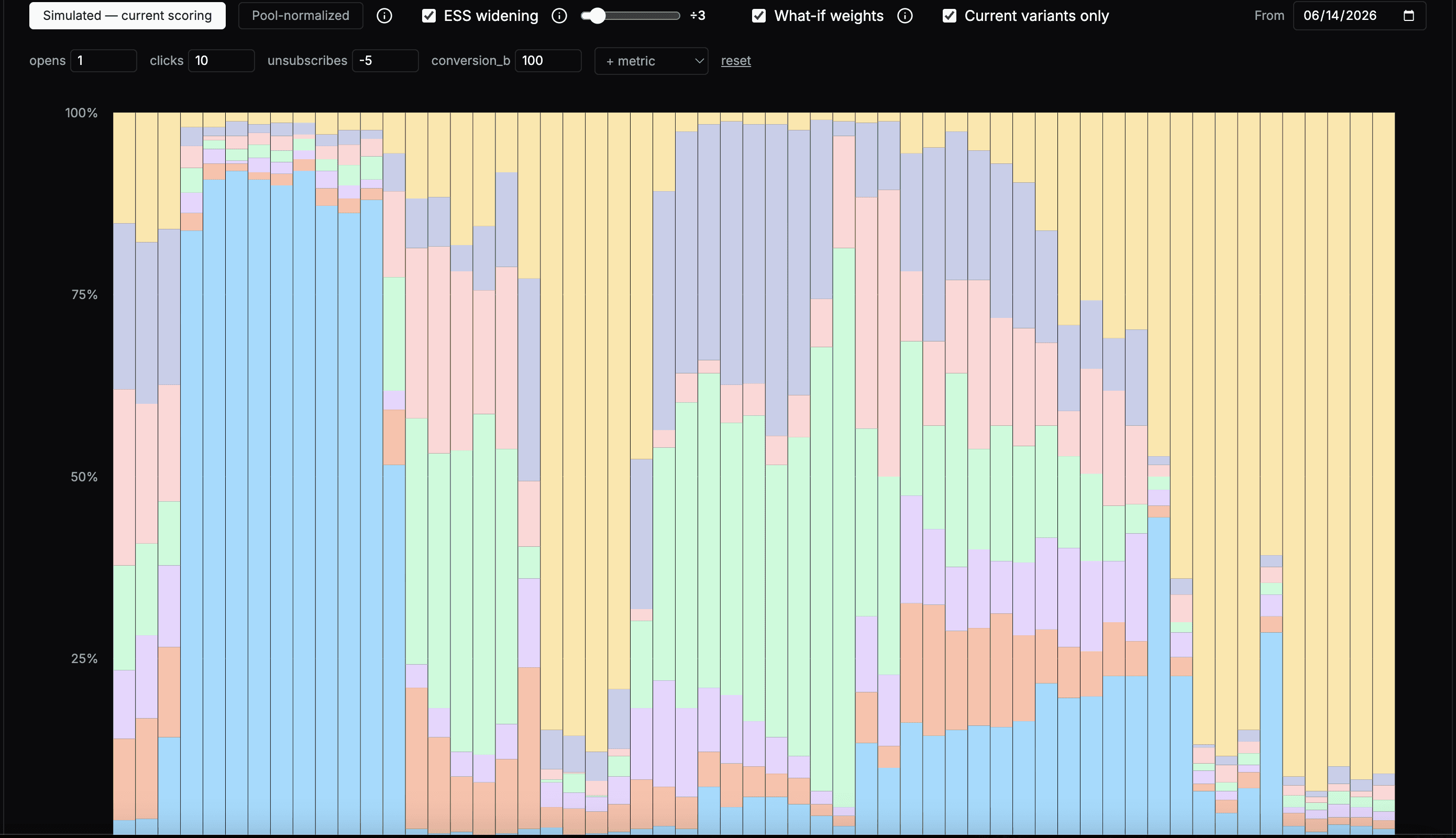
Figure 6: Simulated send distribution

Simulated send distribution: each band is a variant's Monte-Carlo win-share per scoring day, replayed over the template's own history; variant names redacted.

That parity is what makes the tool trustworthy: because the mirror reproduces the production scorer step for step, every replay and every OPE number in this post inherits its credibility from it. On one hypersegmented template the reconstructed win-share landed at 33.9% against an actual 33.4%. A simulator that drifted from prod would be grading a policy that never ran.

Catching the next one: a closed loop

Fixing templates by hand does not scale, so we built a loop that catches the next degradation on its own: detect, grade, confirm, apply. Everything up to the last step is read-only, and a human takes the last step.

Detect. The published approach (M-UCB, CUSUM-UCB) puts change detectors on each arm’s reward stream inside the algorithm. We watch the allocation stream from the outside instead. Every shape signal alone false-alarms on a healthy bandit: low entropy is just successful exploitation, and high churn is often legitimate rotation. So a finding fires only on a conjunction of a shape signal and a harm signal. The building blocks are normalized allocation entropy⁶ (dividing by ln n for n variants rescales it to 0–1) and total-variation churn over the daily send-share vector p, whose entry p_a is variant a’s send share:

Entrenchment fires only when concentration coincides with a wrong leader; whipsaw only when thrashing coincides with enough volume to matter:

Figure 7: Entropy and the entrenchment gate

Concentration alone is not harm: the entrenchment gate crosses low entropy with a wrong-leader check.

The rank is read off matured, prior-pinned posteriors (rates from windows old enough for conversions to have landed), so concentration onto a genuinely-best arm never fires, and churn is measured only across day-pairs whose competitive roster is unchanged (that roster guard alone killed 45 of 49 apparent whipsaw windows on one template). A finding must persist across at least three windows, a cheap stand-in for always-valid inference (confidence sequences) that holds the false-alarm rate under control across repeated looks at the same stream. The whole detector is regression-pinned to real fixtures: it fires on the ground-truth incident before the fix, goes silent after, and stays quiet on labeled false positives.

Grade. A fired finding routes to its lever, and we grade it before shipping with the cheapest valid estimator. Off-policy evaluation from logs is unbiased under correct propensities and overlap (every action the proposed policy would take had a nonzero chance of being logged, so nothing it does is invisible to the data): inverse-propensity scoring reweights each of the n logged decisions by the importance weight w_i = π_e(a_i)/π_b(a_i), the ratio of the proposed policy’s probability of the logged action to the logging policy’s own. Decision i carries a logged action a_i and a matured reward r_i. Raw IPS is unbiased but high-variance, so we never grade on it directly; the self-normalized form (SNIPS) divides by the summed weights, trading a small finite-sample bias for far lower variance:

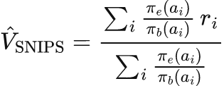
The estimate we act on is the doubly-robust one⁵: it corrects a fitted reward model r̂(a) with that same importance weight w_i and is unbiased if either the weights or the model is right. We report SNIPS beside it as a model-free cross-check. DR leans partly on the reward model and SNIPS on none, so when the two agree the number is not an artifact of either:

We trust neither blindly. We gate on the Kish effective sample size; when the proposed policy diverges from what ran, one decision’s weight dominates, the effective sample size collapses toward 1, and the estimate is a single sample in disguise:

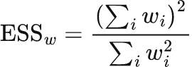
We ship a change only when DR’s interval excludes zero, SNIPS agrees, and the weight-ESS is healthy. A small change clears this from logs; a large one collapses the ESS and falls back to replaying the change over the template’s real history against a reserved holdout. The weight-ESS decides which engine is valid, so the choice is mechanical.

Confirm, then apply. Grading only screens. A randomized ~10% holdout the bandit never touches is what identifies the causal effect rather than the bandit’s own selection. Only the last step mutates config, and a human takes it.

Results

Every row shipped. The headline change was confirmed on a live randomized holdout, the causal gold standard; the rest by replay over each template’s own real traffic, on a mirror validated against the production scorer to within 0.5 points.

What ties these together is the loop underneath: a map from symptom to lever, a grader that picks the right estimator for the size of the change, a toolkit that makes every contest inspectable, and a monitor that catches the next distribution shift and feeds it back in. The result is a repeatable program in place of one-off firefighting.

Notes

¹ ESS widening. Dividing both parameters of a variant’s Beta distribution by the same constant. It widens the distribution, adding uncertainty and exploration, without moving its mean, so a starved variant gets sampled again while its estimated rate stays put.

² Pool normalization. Rescaling each day’s counts so the whole pool’s conversion rate is pinned to its median across days. It cancels day-to-day swings that would otherwise reward a variant just for being shown on a high-converting day.

³ Empirical-Bayes partial pooling. Estimating each segment from a blend of its own data and the campaign-wide average, leaning on the average when the segment has little data of its own, so small segments borrow strength instead of guessing.

⁴ Minimum detectable effect (MDE). The smallest real improvement an experiment has enough data to catch reliably. If a metric’s MDE needs more events than a campaign will ever see, it cannot be optimized as a target.

⁵ Doubly-robust estimation. A way to estimate how a not-yet-deployed policy would perform that stays accurate if either the reweighting or a simple reward model is right, giving two chances to be correct instead of one.

⁶ Allocation entropy. One number for how evenly traffic is spread across variants: high when it is shared broadly, low when a single variant dominates.

References

Thompson sampling. Thompson (1933); Chapelle & Li (2011); Agrawal & Goyal (2012, 2013); Russo (2016), Top-Two Thompson Sampling.

Exploration and non-stationarity. Sutton & Barto (2018); Garivier & Moulines (2011), discounted and sliding-window UCB; Cao et al. (2019), M-UCB; Liu et al. (2018), CUSUM-UCB.

Off-policy evaluation. Horvitz & Thompson (1952), IPS; Swaminathan & Joachims (2015), SNIPS and CRM; Dudík, Langford & Li (2011), doubly robust; Kish (1965), effective sample size; Saito et al. (2020), Open Bandit Pipeline.

Empirical Bayes and shrinkage. Efron & Morris (1975), Stein estimation; Gelman & Hill (2007), partial pooling.

Contextual bandits. Li et al. (2010), LinUCB; Agrawal & Goyal (2013), Thompson sampling for contextual bandits.

Multiple comparisons and sequential validity. Benjamini & Hochberg (1995), FDR; Johari et al. (2017/2022), always-valid inference; Howard et al. (2021), confidence sequences.

Reward centering (pool-normalization framing). Krishnamurthy et al. (2018), context-centering to cancel a confound; Naik et al. (2024), Reward Centering.